Time series storage

Time series data is stored in a container unless the data remains small enough to fit in a single row of a table. When a time series is stored in a container, the data is stored contiguously and is retrieved with a minimum number of disk reads. If you do not create time series containers before you insert time series data, the containers are created automatically as needed. You can manage storage by controlling in which dbspaces the time series data is stored and by deleting old time series data.

You can store only 1500 bytes of time series data in-row. Containers store the data outside of the database table. The row in the table contains a reference to the container. If you copy the data in the table, you do not copy the data in the container. Instead, you create a second reference to the data in the container. For example, the following statement copies the table and adds a second reference to the container:

INSERT INTO tab2 SELECT * FROM tab1;

You control how many elements are stored in-row by setting the in-row threshold when you create a time series. You can specify that all time series elements are stored in containers by setting the in-row threshold to 0.

Containers

A container is mapped to a disk partition in a dbspace. A dbspace is a logical grouping of physical storage (chunks). The following illustration shows the architecture of containers in the database. A database usually contains multiple dbspaces. A dbspace can contain multiple containers along with tables and free space. A container can contain data for one or more sources, for example, electricity meters. The time series data for a particular source is stored on pages in time stamp order.

The graphic is described in surrounding text. — Figure 1: Architecture of the default configuration of a container in a databaseArchitecture of a container in a database

When you insert data into a time series and you do not specify a container name, the database server checks for one or more containers that are configured for the time series. If any matching containers exist, the container with the most free space is assigned to the time series. If no matching containers exist, the database server creates a matching container in each of the dbspaces in which the table is stored. For example, if a table is not fragmented and is therefore stored in a single dbspace, one container is created. If a table is fragmented into three dbspaces, three containers are created.

All containers that are created automatically by the database server belong to the default container pool, called autopool. A container pool is a group of containers. You can create one or more container pools in which to include containers. You can assign containers to container pools. Alternatively, you can create your own container pool policy function.

Strategies for using multiple dbspaces with containers

Strategies for storing time series data in multiple dbspaces depend on how the data is distributed, how data is inserted into the appropriate container, and how you delete old data.

Time series data is stored in multiple dbspaces in the following situations:

The table is fragmented over multiple dbspaces and containers are created automatically in the same dbspaces as the table fragments.
You create multiple containers in multiple dbspaces.
You create a rolling window container that stores time series data in multiple dbspaces.

The following table compares the different strategies.

Table 1. Comparison of container strategies
Strategy	Data distribution method	Inserting data	Deleting data by date range
The table is fragmented among multiple dbspaces and containers are created automatically.	The time series data is distributed among the same dbspaces as the table fragments.	The data is stored in containers in round robin order.	You run the TSContainerPurge function to delete data by date range in all containers.
You create multiple containers in multiple dbspaces.	You decide how to distribute the data. You can distribute the time series data by primary key values. You can decide on a specific set of primary key values for each container.	You specify the appropriate container name for the primary key values when you insert data.	You run the TSContainerPurge function to delete data by date range in all containers.
You create a rolling window container.	The time series data is distributed by date interval. Each date interval is stored in its own partition. Partitions are stored in multiple dbspaces.	You specify the rolling window container name when you insert data. The container controls in which dbspace the data is stored.	You configure an automatic purge policy to delete data by date range, or you manually destroy partitions.

Multiple dbspaces for multiple containers

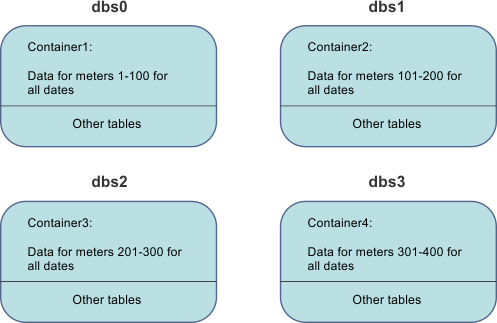
The following illustration shows multiple containers in multiple dbspaces. The time series data is distributed by the primary key value.

Each container stores the data for all dates for a specific set of meter IDs. Each dbspace stores a container and other tables. If the containers were created automatically, each dbspace contains the table fragment that stores the same primary key values as the container.

Dbspaces for a rolling window container

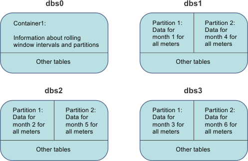
When you create a rolling window container, you specify a time interval by which to store the data and the list of dbspaces in which to store the data. A rolling window container stores time series data by the specified time interval in separate partitions. Partitions are stored in the specified dbspaces in round robin order. The container dbspace stores the information about what data is in which partition. The following illustration shows a container that stores data in four dbspaces. The time interval for each partition is one month.

In this illustration, the dbspace named dbs0 contains the container, Container1, and other tables. Container1 stores the information about the time interval of the data in each partition and the location of each partition. The dbspaces named dbs1, dbs2, and dbs3 store time series elements in partitions and other tables. Each partition stores the data for one month for all meter IDs.

Active and dormant windows

Partitions make it easy to remove old data. You can configure a rolling window container to automatically delete old data after a specified amount of data is stored. You specify the number of partitions to keep in the active window and in the dormant window. The active window contains the partitions into which you can insert data. The dormant window contains partitions that you no longer need to query, but are not yet ready to delete. The active window moves ahead in time when you insert data for the next time interval. When you insert data that is after the latest partition, a new partition is added and the active window moves ahead. When the active window exceeds the maximum number of partitions, the oldest partition is moved to the dormant window. When the dormant window exceeds the maximum number of partitions, the oldest partition is destroyed.

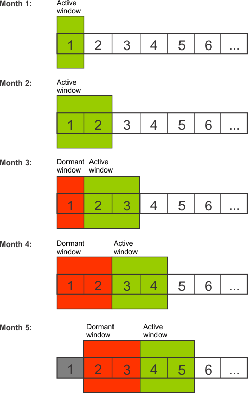
The following illustration shows how an active window and a dormant window grow and move over time. In this example, the maximum size of both windows is two months.

This illustration shows how the windows grow and move as data is inserted for each month:

When data is added for month 1, a partition is created in the active window.
When data is added for month 2, a second partition is created in the active window.
When data is added for month 3, the partition for month 1 moves out of the active window and into the dormant window.
When data is added for month 4, the active window adds a partition for month 4 and moves the partition for month 2 into the dormant window.
When data is added for month 5, the active window and the dormant window move forward. The partition for month 1 is destroyed.

You can move partitions between the active and dormant windows and change the size of the windows.